Better Understand Your Data: Freeze & Re-Size Excel Header Rows & Columns
When your Excel spreadsheet is full of rows and columns, it can get difficult to browse. You use it to store important data, from business revenue to sales or customer information to… who knows, maybe a list of locations. To get the most from your spreadsheets, you want to be able to connect each piece of data with key labels. None of your rows upon rows of data are quite as important as your header row, which can help keep your data organized.
In this post, we’ll show you how to keep your most important data visible while you browse your spreadsheet. Read on to see how to freeze rows (like a header) in Excel, along with some more Excel row tricks, including how to automatically re-size rows to fit your data. Let’s get started.
Add & Freeze Header Row(s)
Excel can hold over a million rows of data. While this is great for anyone with big datasets, it also makes it easier to forget the value of row 123,456. It’s a huge time-saver to be able to see that header row—or any other important rows—at all times. Thankfully, you can modify the worksheet so the first row is always visible when you scroll the worksheet down. To add and then freeze a header row in Excel:
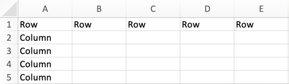
- Right-click on Row 1 and click Insert
- A new row will appear above your data where you can type your header in each new cell
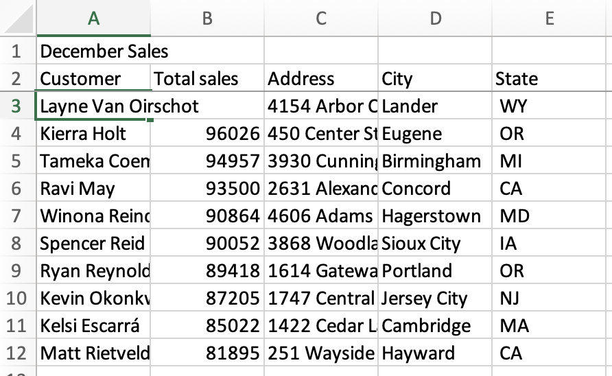
- For example: Customer, Total Sales, Address, City, and State
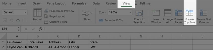
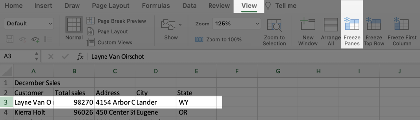
- Navigate to the View tab and select Freeze Top Row
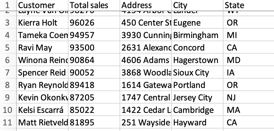
Wherever you scroll, your header row will remain in place. To freeze more than just the first row, follow the steps above. The only change is to select the row beneath the last row you’d like to freeze (i.e., we wanted to freeze the first two rows, so we selected row three). Then, opt for Freeze Panes instead in the View tab to freeze all of the rows above the row you selected.
To freeze a column, select Freeze First Column. For multiple columns, click on the column to the right of where you’d like to freeze, then select Freeze Panes. Now we can move on to another column-related trick that also helps us better understand our data.
Interactive Maps Made Easy
Sign Up NowAutomatically Re-Size Columns to Fit Your Data
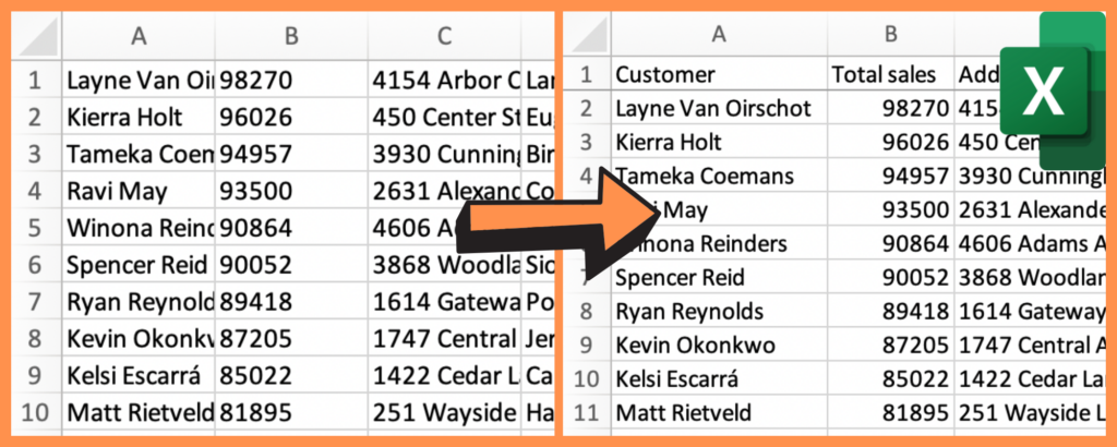
Even with your header row(s) and columns in place, getting the gist of your data at a glance can be hard when some data points naturally take up more space in a cell. For example, it would be nice to see the full name of each Customer without needing to click into the cell. It’s immensely helpful to change the width of your columns so that the contents automatically fit within the column, which we can do in Excel. Follow these steps:
- Select all of the columns you’d like to re-size
- Double-click one of the lines that separates the columns
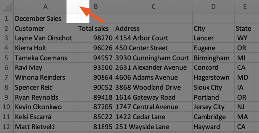
Every column you selected will automatically be re-sized to fit the longest data point, allowing you to see it all.
If you only care to see part of a cell’s data (such as a Customer’s first name), you can also manually re-size individual columns by once again clicking the line that separates each column and dragging it larger or smaller. For now, let’s move on to one final thing you can do to help you better understand the relationship between your data.
Visualize Your Data with a Map

We’ve gone from a spreadsheet with no headers and columns that don’t fit the data to a sheet with clear headers that remain at the top no matter how far down you scroll. Let’s take it one step further by mapping our data to truly see the relationship between our data’s location like address, city, or state and the rest of its columns.
View December Sales in a full screen map
You’ll be able to see your location data (think addresses, cities, states, ZIP codes, countries, geographic coordinates, and even landmarks) plotted on a customizable Google Map. Any additional data (in our case, Total sales) will automatically be grouped together, enabling you to filter the map by only what you want to see. Whether that’s the highest or lowest sales or any other insights, is up to you. Here’s how to do it:
- Open your spreadsheet
- Select (Ctrl+A or Cmd+A) and copy (Ctrl+C or Cmd+C) your data
- Open your web browser and navigate to batchgeo.com
- Click on the location data box with the example data in it, then paste (Ctrl+V or Cmd+V) your own data
- Check to make sure you have the proper location data columns available by clicking “Validate and Set Options”
- Select the proper location column from each drop-down
- Click “Make Map” and watch as the geocoder performs its process
Map your location data today at batchgeo.com.