Calculating Change Between Years in Excel
If you own a business or your job has anything to do with sales, you likely have all sorts of information about your customers or leads. But are you making the most of this data?
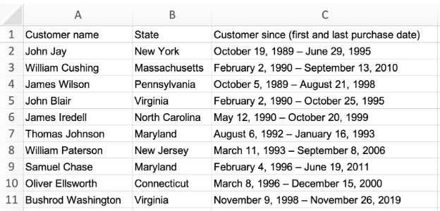
If you store this information in Excel or another tool that can export a CSV file, you may be overlooking key metrics that could help improve your company, such as dates. For example:
- First purchase date
- Last purchase date
You can make more of the data you have by going from this…
…to this!
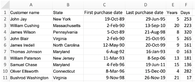
When you separate dates in Excel, you can sort your data by year, month, and day, making it easier to find patterns. You can also use Excel to compare dates, determining the duration of the engagement you’re measuring.
We used the following tips to split data of the birthdates and tenures of 115 US Supreme Court Justices, which is why the customer names in our examples may sound familiar. So, let’s get started with Excel’s formulas and features.
Split Dates into Sortable Days, Months, and Years
Say you have a cell that contains year, month, and day — this may not be the best format if you’re trying to isolate the most common months.
There are many ways of separating dates into unique columns in Excel, but perhaps the easiest is using “Text to Column.” Google Sheets has a similar feature. Here’s how to do it in Excel:
- Select the cells you’d like to separate.
- Navigate to the “Data” tab.
- Select “Text to Columns…”.
- Choose whether your data is currently separated by Delimited characters such as commas or colons or Fixed width with spaces between each field (we usually opt for the first).
- Click “Next” and either check off the delimiters your data contains (tabs, semicolons, commas, spaces, or you can customize any other delimiter, such as backspaces or hyphens) or set the column breaks.
- Select “Next” and choose where you want your separated data to end up.
- Click “Finish,” and you’re done!
Now that you’ve separated days from months and years, you can sort the individual columns or use pivot tables to count and summarize. You can also use an Excel formula to compare dates.
Interactive Maps Made Easy
Sign Up NowCalculate the Time Between Two Dates
You have two dates split into individual columns in Excel. Some data analysis requires you to calculate how many years, months, or days are between them. Below is the simple Excel formula that allows you to do this:
=DATEDIF(Start_date, End_date, Unit)
- In a new column, start by typing “=DATEDIF(“
- Follow up by either clicking the cell with your start date or typing in its corresponding letter and number (i.e., D2) followed by a comma.
- Now, click your end date or enter it in (i.e., E2), again followed by a comma.
- Next, in quotations, specify whether you want the time between the two dates to be in days, months, years, or some combination.
- “d” is used for the difference in days
- “m” means the difference in complete months
- “y” is for the difference in complete years
- Close your parentheses.
Note: There are also ways to exclude data, such as:
- “md”: Difference in days, excludes months and years
- “ym” : Difference in months, excludes years
- “yd”: Difference in days, excludes years
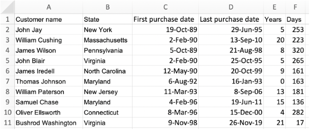
For our purposes, we want only the years and days between our two dates so we used two formulas in two columns, “Years,” and “Days.”
=DATEDIF(D2,E2,“y”)
and
=DATEDIF(D2,E2,“yd”)
Drag it down all your rows, and you’ll automatically calculate the difference!
Map Your Data and Dates
With your data organized and some Excel math under your belt, let’s see how you can get the most out of your spreadsheet. Plotting your points on a custom map is the natural next step if your data contains locations, such as addresses, cities, or states.
There are quite a few ways to do this, from desktop GIS software like ArcGIS or a Google Maps API, as explained in Introduction to Map Making on the Web. But the easiest method is to use Batchgeo, a dedicated tool that geocodes your location data. Here’s how to make a map with our free geocoder:
- Open your spreadsheet.
- Select (Ctrl+A or Cmd+A) and copy (Ctrl+C or Cmd+C) your data.
- Open your web browser and navigate to batchgeo.com.
- Click on the location data box with the example data, then paste (Ctrl+V or Cmd+V) your data.
- Ensure you have the proper location data columns by clicking “Validate and Set Options.”
- Select the proper location column from each dropdown.
- Click “Make Map” and watch as the geocoder performs its process.
Thanks to splitting our data and our date math, our map looks like this:
View Sales Data with Dates (After) in a full screen map
Otherwise, it would have looked something like this:
View Sales Data with Dates (Before) in a full screen map
Check out our other Excel tips to upgrade your spreadsheet game even further:
- How to Find Duplicates in Excel
- Excel Data Visualization Examples
- Simplify Complicated Data in Excel Spreadsheets
Or get mapping today for free at batchgeo.com.