Tired of manually inputting numbers into every cell of an Excel Workbook just to have to do it again the following month? How about trying to track down that one shipping number that just doesn’t seem to exist no matter how many times you check each row? Well my friend, what if I told you that you can do ALL of those things and MORE with what is already built into Excel? Over the course of the following pages, we’ll be looking into some unique functions that can not only speed up your workflow by searching with Vlookups or Index Match Arrays but also enhance the accuracy of your work with Left, Right and Mid as well as Count! Well what are you waiting for, let’s dive right in!

Here’s a preview of what we cover below:

• Get Some Quick Analysis with COUNTIF
• Combine Cells Together With CONCATENATE
• Find Substrings with LEFT, RIGHT, and MID
• Extract Related Data With INDEX and MATCH
• Quickly Reference Other Cells With INDIRECT
• Create a quick and easy reference check using VLOOKUP and HLOOKUP
• Transform data formats with TRIM, VALUE, and TEXT

Get Some Quick Analysis with COUNTIF

Excel’s count functions are great time savers and tools to use when building more complex compound functions. On their own, they are also extremely useful to quickly get a count of the number of values in a row or column.

At a base level, all COUNT functions do exactly what their name states, count! However. The count formula you use will vary depending on your needs. In the following, we’ll cover COUNT, COUNTIF,and COUNTA

COUNT

The COUNT function counts the number of cells that contain number values. It will NOT count cells containing text values without a special addition. To COUNT text values, see COUNTIF or COUNTA below.

=COUNT(Value Range, Value Range 2, Value Range 3, ETC)

Value Range(s) can be defined as any set range within Excel. You can select either a vertical, horizontal or combination of the two to create a value range to count.

• For example
  • =COUNT(A1:A12) – Column Only
  • =COUNT(A1:D1) – Row Only
  • =COUNT(A1:D12) – Row And Column Combination
    

Further, multiple value ranges can be selected.  For example, if you needed to count values from both A1 – A12 and B1 to B12, you can use the formula: =COUNT(A1:A12, B1:B12).

This will return a count of every number value within BOTH number ranges. You can add up to 255 additional ranges, but at that point, a better function may be needed.

COUNTA

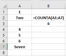
The COUNTA function counts cells that are not empty. This means, unlike the COUNT function, you can count cells with both text and number values in it.

=COUNTA(Value Range, Value Range 2, Value Range 3, ETC)

Outside of what it is able to count the rules are the same for how it is defined.

Value Range(s) can be defined as any set range within Excel. You can select either a vertical, horizontal or combination of the two to create a value range to count.

• For Example
  • =COUNTA(A1:A12) – Column Only
  • =COUNTA(A1:D1) – Row Only
  • =COUNTA(A1:D12) – Row And Column Combination
    

Further, multiple value ranges can be selected.

If you needed to count cells that are not empty from both A1 to A12 and B1 to B12, you can use the formula: =COUNTA(A1:A12, B1:B12).

This will return a count of every cell that is not empty within BOTH number ranges. You can add up to 255 additional ranges.

COUNTIF

COUNTIF  is one of the more useful counts as it allows you to specify a range then a criteria for what you’d like to count. For instance, you can count how many Yes or Nos are in column B with 2 countif formulas that are accurate and precise.

=COUNTIF(RANGE,CRITERIA)

The RANGE can be a column, a row, a combination of both or even a table. The range defines where you are looking to count in.

• =COUNTIF(A1:A12,CRITERIA)
  

The CRITERIA for a COUNTIF function is a little more vague. It is very customizable but without knowing what can be entered, can be rough for newcomers.

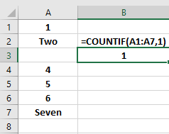
• • • It can be a number value. For example, looking for the number 2 in the range

• =COUNTIF(A1:A12,2)
  
  • It can be a text value. For example, looking for the word Hello in the range
• =COUNTIF(A1:A12, “Hello”)
  
• • • It can even be used to find cells with no values within them
• =COUNTIF(A1:A12, “”)
  

Sample Count Function Formulas

COUNT

• • Count the number of today’s sales in range B1:B12 and multiply them by the average sales price in Cell C3.
    • =COUNT(B1:B12)*C3
  • Count the number of weekly sales in range A1:A12, B1:B12, C1:C12, D1:D12,E1:E12 and multiple them by the average sales price in Cell F3. Once multiplied, increase product by 5% to show growth.
    • =(COUNT(A1:A12,B1:B12,C1:C12,D1:D12,E1:E12)*F3)*1.05)
      OR
    • =(COUNT(A1:E12)*F3)*1.05
      

COUNTA

• • After combing through your shared workbook, you realize that 100 people have used a combination of both text and number fields when entering their data in range B1:B3000. You need a count of these values but COUNT is no longer accurate as you are only counting NUMBER values and not cells that have information filled. You can now use COUNTA instead.
    • =COUNTA(B1:B3000)
  • Formula to confirm that worksheet WORKSHEETA has an equal amount of data filled in worksheet WORKSSHEETB in range A1:A600 regardless of it is number values or not.
    • =IF(COUNTA(‘WORKSHEETA’!A1:A600) = COUNTA(‘WORKSHEETB’!A1:A600), “YES”, “NO”)
      1. This formula will return a YES if the values in the range on both worksheets are equal. If they are not, it will return a NO
         

COUNTIF

• • If the number of Yes responses counted within range A1:D20 are less than 10, the text will read Fail. If it is equal to 10 or more, it will read Succeed

• • • =IF(COUNTIF(A1:D20, “Yes”)>=10, “Succeed”, “Fail”)
  • Count then add the number of Yes, No, and Undecided responses in range A1:A20
    • =COUNTIF(A1:A20,”Yes”)+COUNTIF(A1:A20,”No”)+COUNTIF(A1:A20,”Undecided”)

Combine Cells Together With CONCATENATE

Stop me if you’ve heard this one. You’ve been tasked with making a list of a group of people and you’ve been given the first name and last name in two separate columns. The only issue is your company needs them all as one name in one column to make it accurate. Normally, this would be a long process of making a new entry in each cell but with CONCATENATE, your precious time will be saved.

CONCATENATE

The CONCATENATE function can be used to combine multiple cells into one cell without any manual work on your end. As long as there is some kind of value within the cell, and not an error, you can combine it with CONCATENATE

=CONCATENATE (Text1,Text2,Text3,Text4,Text5,Text6)

The TEXT fields above can be set to reference any cell or you can manually input a number, symbol, or word that you want to be added into the combination

• =CONCATENATE(E3,E4)

• =CONCATENATE(E3,”!”)
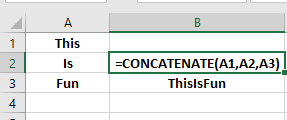
• =CONCATENATE(E3,E4,”Fun”)

The TEXT fields are always added in the order you put them in. For the above examples, if the word This was in E3 and Is was in E4 then you would get the following returns where you use the formula.

• • ThisIs
  • This!
  • ThisIsFun
    

As mentioned earlier, we can put another character anywhere we want, so we can enhance the formulas above with better criteria to space them out into a more readable format.

• =CONCATENATE(E3,” “,E4)
• =CONCATENATE(E3, “-” “!”)
• • =CONCATENATE(E3,”-“,E4,”-“,”Fun”)

Which returns

• • This Is
  • This !
  • This-Is-Fun
    

Sample Concatenate Formulas

A formula that counts the combined text values of E3 and E4 in range A1:A20

• • =COUNTIF(A1:A20,CONCATENATE(E3,E4))
    

A formula that combines first name from Cell A1, Middle name from Cell B1, and Last name from Cell C1 with a space between each name and in the format of Lastname,FirstName Middleintial. Just for fun, we’ll also add a TRIMs which removes any excess spaces from the starting data so you get a nice clean result.

• • =CONCATENATE(TRIM(C1),”,”,TRIM(A1),” “,TRIM(B1),”.”)

Find Substrings with LEFT, RIGHT, and MID

Spreadsheet data can be entered in a wide variety of ways but once it hits a point where you have multiple worksheets comparing and contrasting different values, it’s hard to go back and rewrite a couple hundred rows of values to increase accuracy or make a formula work right. LEFT, RIGHT, and MID however help you get into the thick of things with a great way to grab just a bit of data instead of the whole segment to compare with.

LEFT

The LEFT function returns the first character or characters in a text string, based on the number of characters you specify. This is a direct quote from the Office site and defines it so well that it’s hard to dispute.

=LEFT(TEXT, Number of Characters)

The TEXT field is a bit of a misnomer, you specify a cell and it returns the string of characters within it. This can be done on a group of numbers or a group of text.

• =LEFT(A1,Number of characters)

• =LEFT(50192,Number of characters)
• =LEFT(“Excel is fun”,Number of characters)

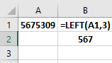
Once you place your text, you would then define the number of characters you’d like to display starting at the left of the string

• • Entering =LEFT(50192,1) into cell A1 would display 5
  • Entering =LEFT(50192,5) into cell A1 would display 50192
  • Entering =LEFT(50912,3) into cell A1 would display 501

RIGHT

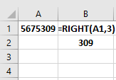
The RIGHT function is similar to the LEFT however it starts at the end of the string instead of the beginning.

=RIGHT(TEXT,Number of Characters)

The TEXT Field for RIGHT is identical to the LEFT function. You can specify a cell or a string and it will use that value as its starting point.

• =RIGHT(A1,Number Of Characters)

• =RIGHT(50192,Number Of Characters)
• =RIGHT(“Excel is fun”,Number Of Characters)

Once you place your text, you would then define the number of characters you’d like to display starting at the right of the string

• • Entering =RIGHT(50192,1) into cell A1 would display 2
  • Entering =RIGHT(50192,5) into cell A1 would display 50192
  • Entering =RIGHT(50912,3) into cell A1 would display 912
    

MID

The MID function is different from LEFT and RIGHT as it starts where you specify and then will use that to move left from there.

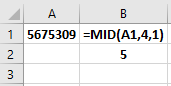
=MID(TEXT,Starting Character,Number Of Characters)

The TEXT Field for MID is identical to the LEFT and RIGHT functions. As a reminder, you can put a cell reference or specify text or a number within it.

• =MID(A1,Starting Character,Number Of Characters)

• =MID(50192,Starting Character,Number Of Characters)
• =MID(“Excel Is Fun”,Starting Character,Number Of Characters)

The Starting Character requires a bit more work to determine. If using the phrase Excel is Fun as our starting point and want to return on the Is of the word, we’d want to write it as:

• =MID(“Excel Is Fun”,7,Number of Characters)
• • • The word Excel counts as 5 characters
    • The space between Excel and Is counts as 1 character
    • We want to start at character number 7 to grab the first letter of Is
      

Once you have your text and starting character, you would then enter how many characters from the starting point to display. Remember, this counts from the left similar to the LEFT function.

• Entering =MID(50192,3,1) will return 1

• Entering =MID(50192,1,5) will return 50192
• Entering Entering =MID(50192,3,2) will return 1 will return 19

Sample LEFT, RIGHT, and MID Formulas

LEFT

• A formula to grab the 5 digit number value starting from left to right in cell A3 then use the result to count how many times the code appears in range B1:B20
  • =COUNTIF(B1:B20,LEFT(A3,5))
• A formula mixed with the Find function to grab everything before the first space in a string located in A2
  • =LEFT(A2,(FIND(” “,A2,1)-1))
    • The FIND function looks for the specified criteria, in this case a space, within the string you are within, A2, starting at the character you specify,1. Once it locates the space, the LEFT function grabs the string from the beginning to that space. This is invaluable when needing to split up data that is written all together. You can swap the ” ” for “-” to look for hyphens or other special characters.  
      

RIGHT

• A formula that returns only the last 3 digits of a VLOOKUP looking for the value in A2 within the range of C2:F20 and returning the absolute value in column F.
  • =RIGHT(VLOOKUP(A2,C2:F20,4,0),3)
    

MID

• A formula to provide a yes or no if the 3rd, 4th, and 5th number value of a 10 digit string located in cell A2 match the value in cell B2.
  • =IF(VALUE(MID(A2,3,3))=B2, “Yes”, “No”)

Extract Related Data With INDEX and MATCH

Welcome to one of the most complete functions in Excel, INDEX and MATCH. While VLOOKUP and HLOOKUP are great for very specifically organized data, INDEX and MATCH can be used in combination to return almost perfect results with the only limitations being the data stored within the workbook.

INDEX

INDEX comes in two varieties. Array Format and Reference Format.

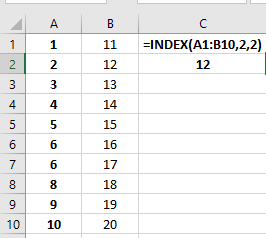
=INDEX(ARRAY,ROW NUMBER,COLUMN NUMBER)

=INDEX(REFERENCE,ROW NUMBER,COLUMN NUMBER,AREA NUMBER)

The top format is the array format which returns the value of a specified cell or array of cells. The bottom format is the reference format which returns the reference of a specific cell. It will return A2 instead of the value in A2 allowing you to create formulas using Index to quickly get references to other ranges.

The ARRAY format is composed as follows:

ARRAY refers to the range of data you are looking to index. This can be a table, a column, or anything in between. This is a required part of this formula.

• =INDEX(A2:D20,ROW NUMBER,COLUMN NUMBER)

• =INDEX(A2:A20,ROW NUMBER,)
• =INDEX(A2:B20,,COLUMN NUMBER)

ROW NUMBER refers to the row containing the data you’d like to index within the array. If an array only has one row, this can be ignored as shown above. The row number is relative to the range selected.

• • • =INDEX(D2:H20,1,COLUMN NUMBER) will refer to ROW 2

• =INDEX(D2:H20,5,COLUMN NUMBER) will refer to ROW 6
• =INDEX(D2:H20,3,COLUMN NUMBER) will refer to ROW 4

COLUMN NUMBER refers to the column containing the data you’d like to index within the array. This is another optional one as if you do not have more than one column within the array, it is unnecessary to add. The column number is relative to the range selected as well.

• • • =INDEX(D2:H20,1,1) will refer to ROW 2, COLUMN D

• =INDEX(D2:H20,5,5) will refer to ROW 6, COLUMN H
• =INDEX(D2:H20,3,3) will refer to ROW 4, COLUMN F

The REFERENCE format is composed as follows:

REFERENCE refers to the cell or group of cells you are looking to reference. If you are referencing more than one range of cells, you will need to enclose it in Parentheses.

• =INDEX(A2:D20,ROW NUMBER,COLUMN NUMBER,AREA NUMBER)
• =INDEX((A2:D20, D21:G40),ROW NUMBER,COLUMN NUMBER,AREA NUMBER)

ROW NUMBER is identical to the ARRAY format. If looking at multiple ranges, the area number will determine where the row number will begin looking. This is optional if working only in a single row.

COLUMN NUMBER is identical to the ARRAY format. If looking at multiple ranges, the area number will determine where the column number will begin looking. This is optional if working only in a single column.

AREA NUMBER is unique to the reference format and is completely optional. Area Number will specify which of the multiple references to begin looking in. If not filled out, it will assume area 1 and your results will reference this.

• =INDEX((A2:D20, D21:G40),ROW NUMBER,COLUMN NUMBER,1) will return values within range A2:D20

• =INDEX((A2:D20, D21:G40),ROW NUMBER,COLUMN NUMBER,2) will return values within range D21:G40

MATCH

Ever wanted to just quickly know if a value is present in one column or row and get a general idea of where it is? MATCH can do just that by returning a position of where it is located in the specified range.

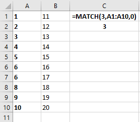
=MATCH(LOOKUP VALUE,LOOKUP ARRAY,MATCH TYPE)

LOOKUP VALUE is the value you want to find within the range. This can be a text input entry, a number or a cell reference.

• • • =MATCH(2,LOOKUP ARRAY,MATCH TYPE)

• =MATCH(“Bacon”,LOOKUP ARRAY,MATCH TYPE)
• =MATCH(E2,LOOKUP ARRAY,MATCH TYPE)

LOOKUP ARRAY is the range of cells you want to search for a match within. Typically, the lookup array will need to be in a column

• • • =MATCH(2,A2:A20,MATCH TYPE)

• =MATCH(“Bacon”,A2:A20,MATCH TYPE)
• =MATCH(E2,A2:A20,MATCH TYPE)

MATCH TYPE is required and needs to be specified to either exact, less than or greater than. Remember how earlier we said that MATCH returns a position when the criteria matches? The results will always either be a number indicating the position or an #N/A which typically means either there are no matches or the formula has issues.

• =MATCH(2,A2:A20,1) will return the position of the value within A2:A20 which is LESS than or equal to the number 2

• =MATCH(2,A2:A20,0) will return the position of the value within A2:A20 which is exactly equal to the number 2
• =MATCH(2,A2:A20,-1) will return the position of the value within A2:A20 which is GREATER than or equal to the number 2

INDEX-MATCH

You got Index in my Match Formula, you got match in my…. You already know the joke. Index and Match are both powerful tools on their own but when combining the two, you can really make a great table searching formula that can make work that much easier. The components are all the same so we are going to go straight into an example instead.

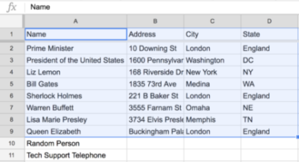
Mark the Shark needs to keep on top of his fish deliveries but can’t seem to locate exactly where a missing order is. In his Array, he needs to first match an exact value located in cell E2 to one in Column C, then pull back the corresponding value in column F. His workbook is laid out in such a way that using a VLOOKUP would have him counting forever and even then, it may not match exactly. He’d like to use an INDEX match to figure it out.

• =INDEX(F2:F20,MATCH(E2,C2:C20,0))
• • When combining index and match, there are a few unique changes that are made.
  • Starting from left to right
    • We start with an INDEX formula and input our ARRAY for the data we want to return
    • For our row number, we use a MATCH formula to specify exactly where we need to go.
    • Since we need to match E2, this is our LOOKUP VALUE
    • Since mark only needs to match an item in Column C, we do not need to specify a LOOKUP ARRAY larger than this.
    • We need the exact item and not something else related to it, so we lock in a 0 for our MATCH TYPE
    • Now that we have our base, next would normally come our column number BUT since we specified only a single column in the ARRAY, we can now ignore this and close out our formula.
  • This will bring back the value in column F that matches the value found in the row set by our MATCH formula

INDEX-MATCH ARRAYS

Building on the previous section, INDEX-MATCH is even MORE powerful when we start setting them into arrays. Arrays are large sets of data where we are looking to pull multiple values, compare them, then produce a result. Index-Match ARRAY formulas are great because we can set multiple criteria to match which make our formulas more able to produce accurate results. The advantage of Index-Match Arrays over other lookups are that we can go 2, 3, or even 4 criteria in and really ensure we are only getting back the results we want.

Let’s start easy with a index match array looking for two criteria

• • • =INDEX(ARRAY,(MATCH(1,(CRITERIA1)*(CRITERIA2),0)))

• ARRAY refers to the range of cells you want a result from
• • • The 1 in the first field of the MATCH is what we are looking for. When running both criteria, if either fails, we DON’T want it to return a match. Anything other than a 1 will result in a failure as it is not unique and more than likely is a duplicate in the workbook.
    • CRITERIA1 and CRITERIA2 refer to what we are looking to.
      • If we need to find A2 in range D2:D20 & B2 in range C2:C20 we would write (A2=D2:D20)*(B2=C2:C20)
      • This forces both criteria to have to match for a result to return, otherwise it will not bring it back.
    • The 0 in our final field is our match type. Data would become unreliable if we are OK with anything less than what we are looking for. We leave it as a 0 to ensure an exact match based on our criteria.
    • Finally, we have no column or cell references here, this is because we are defining them yet again through this method.
  • Sample formula (just for knowing what it looks like)
    • =INDEX(F2:F20,(MATCH(1,(A2=D2:D20)*(B2=C2:C20),0)))
      

When using arrays, once written, you’ll want to confirm addition with CTRL + SHIFT + ENTER on your keyboard. Skipping this step will cause many arrays to fail.

• • When entered correctly, you’ll see: {=INDEX(F2:F20,(MATCH(1,(A2=D2:D20)*(B2=C2:C20),0)))}

Sample INDEX MATCH Formulas

Formula to return a match a value within range A2:A20 and return the corresponding value in column B2:B20

• • =INDEX(B2:B20,(MATCH(A1,A2:A20,0)))

Array with error correction that exactly matches values in range A2:A20 to A1, B2:B20 to B1 and C2:C20 to C1 and returns a value from range D2:D20

• • =IFERROR(INDEX(D2:D20,MATCH(1,(A2:A20=A1)*(B2:B20=B1)*(C2:C20=C1),0))),”No Match”)
    • Don’t forget to hit CTRL+SHIFT+ENTER for accurate results

Quickly Reference Other Cells With INDIRECT

Excel is an odd bird as it doesn’t always like to use references that don’t match its rules. However, INDIRECT allows you to quickly bypass these limitations with its built in functionality.

INDIRECT

The INDIRECT function returns the text value in a cell as a cell reference. It’s useful when used in combination to the Index Reference format formula as once you get the cell reference, you can typically point an indirect at it to have a dynamically changing array.

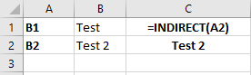
=INDIRECT(REFERENCE TEXT,REFERENCE TYPE)

REFERENCE TEXT refers to the cell reference containing the text you are trying to reference. For this, let’s assume that A2 has the value B2 in it and B2 has the number 12345 within it.

• • • =INDIRECT(A2,REFERENCE TYPE) will return the value of 12345

• =INDIRECT(B2,REFERENCE TYPE) will return a value of #REF!
• • • This is because INDIRECT looks for a cell reference and when it can not resolve it (IE, it cannot find it in the workbook) it will error out and give a reference error.

REFERENCE TYPE is a completely optional statment. It asks for a true or false that translate to A1 or R!C1 style respectively. Unless dealing with Macro references or relative references, you will almost always want to leave this as TRUE or empty.

• • =INDIRECT(A2,TRUE) will return the value of 12345 as A2 is an A1 style reference

Sample INDIRECT Formulas

On WORKSHEET1 you have a list of cell references to values in WORKSHEET2 that do not match what is needed. A formula is needed to quickly trim spaces for values in WORKSHEET2 using cell references in WORKSHEET1

• • =TRIM(INDIRECT(A2))

Create a quick and easy reference check using VLOOKUP and HLOOKUP

When Excel users begin getting more proficient, VLOOKUPS and HLOOKUPS are one of the first power functions they bump into. VLOOKUPS allow a very easy way to find data in other rows, other sheets, or even other workbooks and return a value from a specified column that matches the row it found it in. There are some limitations that we’ll speak about shortly but overall, if you’re looking for a quick and easy way to find and return just about anything; VLOOKUPS are definitely the way to go.

VLOOKUP

The VLOOKUP (or Vertical Lookup) reference function looks in the farthest left column of the LOOKUP RANGE to match criteria set in the LOOKUP VALUE. Once it locates it, it will return a value that matches the column specified in the COLUMN RETURN NUMBER and the row set by the found lookup value with accuracy controlled by the True or False set in the MATCH

=VLOOKUP(LOOKUP VALUE,LOOKUP RANGE,COLUMN RETURN NUMBER,MATCH)

LOOKUP VALUE can be entered as text, a number, or a cell reference.

• =VLOOKUP(“TEST”,LOOKUP RANGE,COLUMN RETURN NUMBER,MATCH)

• =VLOOKUP(12345,LOOKUP RANGE,COLUMN RETURN NUMBER,MATCH)
• =VLOOKUP(A2,LOOKUP RANGE,COLUMN RETURN NUMBER,MATCH)

LOOKUP RANGE is a range of cells set for the function to look through. IMPORTANT. Vlookups ONLY look for values within the leftmost column within a range. If you are looking for a more precision search, see the section on INDEX MATCH formulas above.

• • =VLOOKUP(A2,B2:D20,COLUMN RETURN NUMBER,MATCH) will only look for A2 in column B
  • =VLOOKUP(A2,D2:H20,COLUMN RETURN NUMBER,MATCH) will only look for A2 in column D

COLUMN RETURN NUMBER refers to the relative column number for the value you want to return from your lookup range. Regardless of where your Lookup Range is on the book, you’ll want to count how far your range extends and put in the associated column number.

• • =VLOOKUP(A2,B2:E20,1,MATCH) will return a value from column B
  • =VLOOKUP(A2,B2:E20,3,MATCH) will return a value from column D

MATCH asks if you are OK with an approximate match or a number or value close to what you are looking for. The choices for this Match Type are TRUE or FALSE. Inputting TRUE (or the number 1) will return either the exact value or any value Excel has determined is the largest from the data set but less than your LOOKUP VALUE. Inputting FALSE (or the number 0) will return only exact matches.

• • • NOTE: if your worksheet has multiple matches within it, you will get the first result every time going from top to bottom. When issues like this arise, it’s recommended to look into an INDEX-MATCH ARRAY to add more criteria to your search.
  • =VLOOKUP(A2,B2:E20,1,TRUE) will return the value or the closest value to A2
  • =VLOOKUP(A2,B2:E20,1,FALSE) will only return values that exactly match A2
  • =VLOOKUP(A2,B2:E20,1,1) will return the value or the closest value to A2
  • =VLOOKUP(A2,B2:E20,1,0) will only return values that exactly match A2

HLOOKUP

The HLOOKUP (or Horizontal Lookup) reference function looks in the top row of the LOOKUP RANGE to match criteria set in the LOOKUP VALUE. Once it locates it, it will return a value that matches the row specified in the ROW RETURN NUMBER and the column set by the found lookup value with accuracy controlled by the True or False set in the MATCH

=HLOOKUP(LOOKUP VALUE,LOOKUP RANGE,ROW RETURN NUMBER,MATCH)

I’m sure you noticed but this is extremely similar to the VLOOKUP formula. The only difference is now we’re searching across rows instead of down columns.

LOOKUP VALUE is identical to VLOOKUP. You can enter text, a number, or a cell reference..

• =HLOOKUP(“TEST”,LOOKUP RANGE,ROW RETURN NUMBER,MATCH)

• =HLOOKUP(12345,LOOKUP RANGE,ROW RETURN NUMBER,MATCH)
• =HLOOKUP(A2,LOOKUP RANGE,ROW RETURN NUMBER,MATCH)

LOOKUP RANGE is identical to Vlookup’s as well but typically you’d use an Hlookup if your data is laid out across a row and you’re looking for a value underneath. This is sometimes down when the row labels are in A1 and you are looking across for a specific value then comparing it to value further down the column. IMPORTANT. Hlookups ONLY look for values within the topmost row within a range. If you are looking for a more precision search, see the section on INDEX MATCH formulas above.

• • =HLOOKUP(A2,B2:Z20,ROW RETURN NUMBER,MATCH) will only look for A2 in row 2
  • =HLOOKUP(A2,D2:Z20,ROW RETURN NUMBER,MATCH) will also only look for A2 in Row 2

ROW RETURN NUMBER refers to the relative row number for the value you want to return from your lookup range. Regardless of where your Lookup Range is on the book, you’ll want to count how far your range extends and put in the associated row number.

• • =HLOOKUP(A2,B2:Z20,1,MATCH) will return a value from row 2
  • =HLOOKUP(A2,B2:Z20,5,MATCH) will return a value from row 6

MATCH again is identical to VLOOKUP. Match type asks If you are OK with an approximate match of a number or value close to what you are looking for. The choices for this Match Type are TRUE or FALSE. Inputting TRUE (or the number 1) will return either the exact value or any value Excel has determined is the largest from the data set but less than your LOOKUP VALUE. Inputting FALSE (or the number 0) will return only exact matches.

NOTE: if your worksheet has multiple matches within it, you will get the first result every time going from top to bottom. When issues like this arise, it’s recommended to look into an INDEX-MATCH ARRAY to add more criteria to your search.

• • =HLOOKUP(A2,B2:E20,1,TRUE) will return the value or the closest value to A2
  • =HLOOKUP(A2,B2:E20,1,FALSE) will only return values that exactly match A2
  • =HLOOKUP(A2,B2:E20,1,1) will return the value or the closest value to A2
  • =HLOOKUP(A2,B2:E20,1,0) will only return values that exactly match A2

Sample VLOOKUP and HLOOKUP formulas

A vlookup to find an absolute match of the trimmed A2 text string within range D2:F20 and return the associated value from column F

• • =VLOOKUP(TRIM(A2),D2:F20,3,0)

An Hlookup to find an absolute match of the trimmed A2 within range A2:F20 and return the closest value from row 20

• • =HLOOKUP(Trim(A2),D2:F20,20,TRUE)

A vlookup that uses an hlookup’s return to search within its own range.

• • =VLOOKUP(HLOOKUP(VALUE(TRIM(A2)),D2:E20,5,0),C2:E20,3,0)

Transform data formats with TRIM, VALUE, and TEXT

Excel uses a WIDE variety of different formats ranging from general to custom dates and, unfortunately, they do not play well within some formulas. If you’ve ever made a vlookup that doesn’t return the value you just KNEW was there and later discover the lookup array had spaces in random places (thanks Bob >.>), then here is some piece of mind. TRIM, VALUE, and TEXT can be used to convert strings to what you need and make your life and Bob’s a lot easier.

TRIM

The Trim function removes ANY excess spaces before or after a string to ensure a lookup is accurate. This is a great tool for multiple users all working on a sheet where one person like to add a space behind a name while everyone else doesn’t. It can be added to any formula and helps greatly with accuracy.

=TRIM(TEXT)

The Trim function removes ANY excess spaces before or after a string to ensure a lookup is accurate. This is a great tool for multiple users all working on a sheet where one person like to add a space behind a name while everyone else doesn’t. It can be added to any formula and helps greatly with accuracy.

TEXT works exactly how it sounds. You can either input text into the field or reference a cell.

• =TRIM(”  Excel  “)
• =TRIM(A2)

VALUE

There is a major distinction between a value and text within excel. You can’t add a text and value together in a sum NOR can you do a sum of all text. Similar to trim, we can’t always control how data is put in to a sheet so instead, we make our formulas stronger by adding a VALUE to ensure whatever we add it to is looked at as a value and not a text string.

=VALUE(TEXT)

TEXT works similarly here to TRIM. You can put a reference to a cell here and the formula will turn that into a value

• =VALUE(A2)

TEXT

The TEXT function is actually a bit more unique than most. It can be used at the base level to simply convert values to text but can be enhanced with different format codes to really make your work simplified.

=TEXT(VALUE,TEXT FORMAT)

VALUE either be filled with a number or a cell reference.

• =TEXT(12345,TEXT FORMAT)
• =TEXT(A2,TEXT FORMAT)

TEXT FORMAT refers to a set of format codes that can be used to really customize what is output. Here are a few examples but you can head to Microsoft’s Official Site for more info on format codes: https://support.office.com/en-us/article/number-format-codes-5026bbd6-04bc-48cd-bf33-80f18b4eae68

• • • =TEXT(1234567890,“0”) will return 1234567890

• =TEXT(1234567890,”00000000000″) however will return 01234567890 as we added an 11th 0 which exceeds the total characters in the number.
• =TEXT(1234567890,”###-###-####”) will return 123-456-7890 which is super useful for phone numbers entered as a run on code!

Sample TRIM, VALUE, and TEXT formulas

A formula that removes any excess spaces in the return Column 4 of a vlookup formula looking for the absolute match of A2 in range B2:D20

• • =TRIM(VLOOKUP(A2,B2:D20,4,0))

A formula that trims then converts the return Column 4 of a vlookup formula looking for the absolute match of A2 in range B2:D20 into a value

• • =VALUE(TRIM(VLOOKUP(A2,B2:D20,4,0)))

A formula that trims then converts the return from Column 4 of a vlookup formula looking for the absolute match of A2 in range B2:D20 into a phone number text string

• • =TEXT(TRIM(VLOOKUP(A2,B2:D20,4,0)),”###-###-####”)

Make a Map with Your Newly Gathered Data

Armed with Excel functions that speed up workflow and enhance your work’s accuracy, you can easily gather information like shipping numbers or contact addresses and then make a map of your data. Using our data mapping tool, it’s as simple as copy and paste:

1. Select all of your data columns from your spreadsheet, including the headers
2. Copy the selection using the keyboard shortcut Ctrl+C (Command+C on Mac)
3. Click into the location data box in BatchGeo and paste with Ctrl+V (Command+V on Mac.
4. Click the “Map Now” button and you’re done!