How to Add Inline Charts to Your Maps
Maps tell a story, taking flat data and adding the dimension of location. Similarly, charts and graphs often show data over time. Wouldn’t it be great to blend these together? In this post, we’ll show you how.
View Sales Map for Inline Charts in a full screen map
Take the examples above, two ways of showing customer data. First, the map shows the locations of your top ten customers by sales volume. On the right, you see the same ten, displayed by sales per month over the last year. Each is showing some data that the other isn’t.
Now, consider this merged map:
View Sales Map for Inline Charts with Charts in a full screen map
You can peruse the underlying map data by selecting a field in the lower left. You can see the total sales, for example, to determine which locations are higher than others. Click on each location, and you’ll see the actual sales chart for this location over the last 12 months.
In a single map, you can quickly get the full story, more than is communicated even with the map and chart combined. Let’s walk through how this map was built, and how you can make one with your own data.
Decide Which Data to Display on Your Map
To create a map, the only data you actually need is a set of locations. Technically, a location is described with latitude and longitude coordinates. In practice, an address, postal code, or region name is sufficient. BatchGeo will perform the geocoding to convert location descriptions into coordinates. In addition, any other data you have can be grouped and filtered. Some of this additional data will be what you’ll include in the chart in the next step.
Let’s stick with the sales example above. The sales data and locations of the 10 customers is probably stored in a spreadsheet. You might have a column for the customer name, address, city, total sales, and sales for each of the last 12 months.
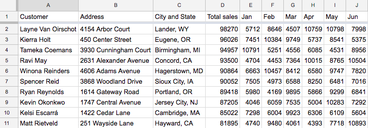
You could put all of this on your map, but only if you expect you’ll want to look at the top customer in June, then turn around and find the top customer in October. More likely, you’re looking for summary data and sales growth. One useful approach could be to calculate the growth rate from the first month through the last month as its own column. Whatever fields you choose to include in your map, keep in mind each one will extend the information box when viewing an individual location. Also, the chart in the next section should provide a much easier view of the monthly data.
Interactive Maps Made Easy
Sign Up NowNote on growth rates: If seasonality could be a factor, you could make sure you have at least 13 months worth of data, so you’re comparing to the same month the year previous.
Let’s say you’ve decided to only show the annual total for each customer. Don’t start deleting data from your spreadsheet. Instead, create a new sheet in the same workbook, or even create new columns to the right of your source data. These new columns will be the ones you use to create your map, so they need to be all together for easy copying. You can use cell references so that if you ever update one set of data, it updates the other.
Generate Chart Image URLs
When we decided what data to include along with the map, we eliminated the individual month data. We want to revive that useful data where it is displayed best: in a simple line chart. By creating chart images for each customer, we can embed it into the information box of each map location.
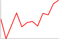
Many charts have a lot of extra labels, a legend, title, and more. Those are important when displaying a chart on its own, because it gives the viewer some context. In this case, we’ll be displaying it alongside other data, so we want to streamline what is displayed. You can play around with creating these charts using this tool. By doing that, I came up with this streamlined chart:
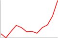
Here we can see simply the change in sales for one customer over 12 months. Now we want to generate those URLs for each of our customers. We can do this dynamically, by inserting our data into the "chd=t:” section of the URL. There’s one thing that makes those chart numbers a little tougher: we need to scale them so each number is between 0 and 100. Since we’re generating this URL in a spreadsheet, that should be fairly each with one gigantic sequence of formulas.
The formula will calculate where each month lies on the scale based on the lowest month being 0 and the highest month being 100. For example, in my spreadsheet the 12 months are columns E (January) to P (December). To find March’s scaled value for the customer in row 2, we use this formula:
=ROUND(100*((G2-MIN(E2:P2))/(MAX(E2:P2)-MIN(E2:P2))), 0)
The result is 17, because March’s $1,401 is closer to the lowest month ($1,190) than the highest ($2,423).
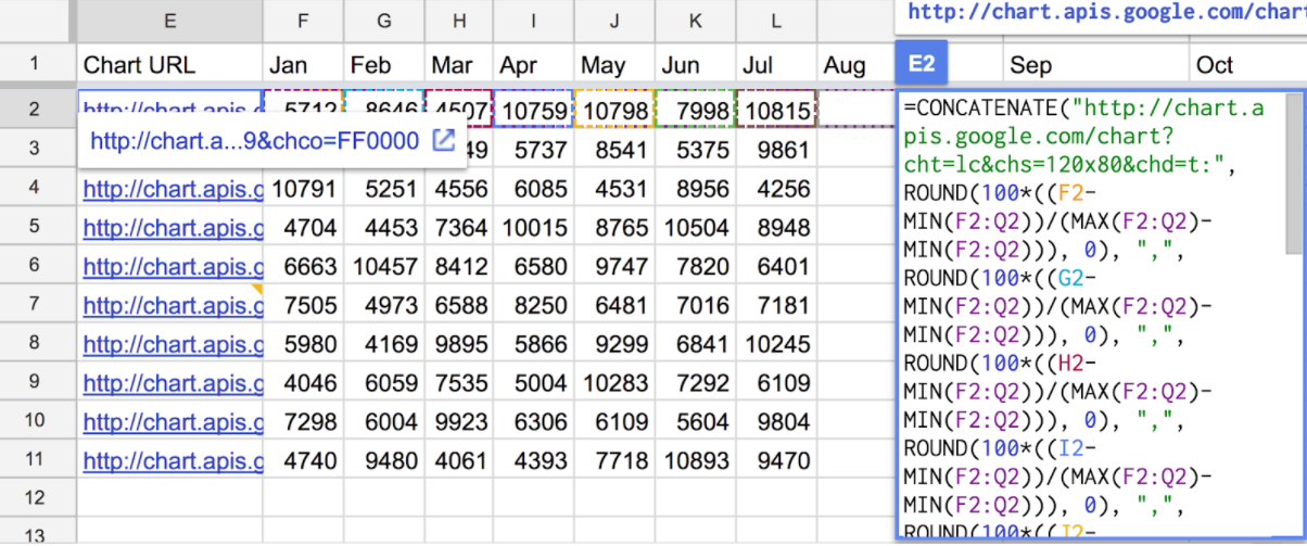
Now we repeat that for each month. Everything above stays the same except the “G2” becomes the column for the appropriate month. We’ll then use CONCATENATE to insert the values into the chart URL. Here’s the complete formula:
=CONCATENATE("http://chart.apis.google.com/chart?cht=lc&chs=120x80&chd=t:", ROUND(100*((E2-MIN(E2:P2))/(MAX(E2:P2)-MIN(E2:P2))), 0), ",", ROUND(100*((F2-MIN(E2:P2))/(MAX(E2:P2)-MIN(E2:P2))), 0), ",", ROUND(100*((G2-MIN(E2:P2))/(MAX(E2:P2)-MIN(E2:P2))), 0), ",", ROUND(100*((H2-MIN(E2:P2))/(MAX(E2:P2)-MIN(E2:P2))), 0), ",", ROUND(100*((I2-MIN(E2:P2))/(MAX(E2:P2)-MIN(E2:P2))), 0), ",", ROUND(100*((J2-MIN(E2:P2))/(MAX(E2:P2)-MIN(E2:P2))), 0), ",", ROUND(100*((K2-MIN(E2:P2))/(MAX(E2:P2)-MIN(E2:P2))), 0), ",", ROUND(100*((L2-MIN(E2:P2))/(MAX(E2:P2)-MIN(E2:P2))), 0), ",", ROUND(100*((M2-MIN(E2:P2))/(MAX(E2:P2)-MIN(E2:P2))), 0), ",", ROUND(100*((N2-MIN(E2:P2))/(MAX(E2:P2)-MIN(E2:P2))), 0), ",", ROUND(100*((O2-MIN(E2:P2))/(MAX(E2:P2)-MIN(E2:P2))), 0), ",", ROUND(100*((P2-MIN(E2:P2))/(MAX(E2:P2)-MIN(E2:P2))), 0), "&chco=FF0000")
That looks mighty complicated, but keep in mind what we’re doing here is to fill in the 12 scaled values to make that chart URL. Excel formulas aren’t known for their brevity, but they get the job done.
Interactive Maps Made Easy
Sign Up NowPut Them All Together
You can use spreadsheet magic to copy the giant formula we created for one customer to all the other customers. The row references in your spreadsheet (E2, F2, etc) should update as you paste (E3, F3, etc). When you have chart images for all the customers, we’re finally ready to make our map.
Using our map making tool, copy and paste all the data you want as part of your map. Be sure to include the header row, the location column, as well as the chart column.
- Paste all the data into the map tool box
- Click Validate & Set Options
- Double check that BatchGeo is using the right columns for the address, city, etc.
- Click Show Advanced Options
- For Image URL, choose your chart URL column
- Click Make Map!
Now check out your map, complete with inline chart!
View Sales Map for Inline Charts with Charts in a full screen map
Click any of the customer markers and you’ll see the data we selected, as well as the chart embedded right there.
You now have a customer map (or whatever data you’ve used) with the data available for filtering, as well as the time series data in an inline chart. Packed into your single map are the many stories in your data.