5 Excel Tips From the Guy Who Built It
Microsoft Excel, and similar spreadsheet software, may be the most used application beyond word processing. Certainly, Excel has a diverse user base and laundry list of use cases, which probably even includes actual laundry lists. Many of us are casual Excel users, and it seems there’s always a new feature to learn.
In a 45 minute video originally shared with his internal teams, former Microsoft Excel Program Manager Joel Spolsky drops gem after gem of Excel knowledge. You can watch the video above and find the top five insights we’ve already put into action in our spreadsheets.
1. Use Tables For More Than Just Pretty Formatting
 You have probably noticed the table feature in Excel. It’s really useful for quickly switching style templates and implementing banded data, where rows alternate in color. In addition to borders and other stylistics, tables also come with some powerful data manipulation abilities.
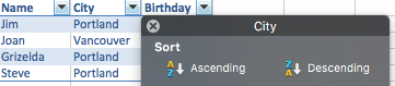
When you use tables, it becomes really easy to sort, sum, and add new data. The formatting is useful for end users, but also helpful in that it signifies to Excel where certain types of data begin and end. Each field in the header row of a table has a dropdown that gives you quick access to sorting and filtering. Fields in the total row let you select from SUM, AVERAGE, and other common Excel functions.
The best part of using tables is how easy it is to add new data. If you include a formula within one cell of a column, it will optimistically be copied throughout the rest of the column. Or, need to add new rows? Simply tab from the last field of the last row and a new row is added above the total row. Sort by a column and the header and total rows stay put. Also, the sorting doesn’t interfere with any other data on this sheet. Everything is contained in its own little world in the table. This becomes especially useful once you name columns and look up data with INDEX, but we’re getting ahead of ourselves.
2. Paste Values to Remove Formatting and Formulas
Interactive Maps Made Easy
Sign Up NowCopying and pasting is the Excel user’s best friend. It makes some powerful assumptions about cell references that make it incredibly useful. However, there are times when what you see is what you want. That’s where Paste Values comes in, a little trick used by Spolsky throughout the session.
For example, you might generate a full name field by using a formula to combine first names and last names (don’t forget the space between). If you later want to remove the first and last name columns, your full name column will disappear… unless you replace it with the values created by your formula.
Try it out:
- Select an entire column that was generated by a formula
- Copy the column to your clipboard
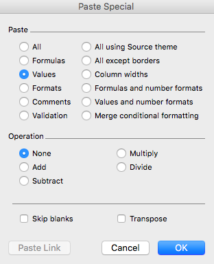
- From the Edit menu, choose Paste Special, then select Values
You can now remove the first and last name columns (or whichever extraneous columns you used to create the column whose values you’ve just pasted). Note that you can also paste formulas, formats (including conditional formatting), and more. Paste Special is, indeed, special.
3. Provide Your Data Room to Breathe
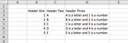 You may notice what first appears to be a strange habit as Spolsky adds data to his spreadsheet. He always leaves Row 1 and Column A blank. Why do cells need room to breathe? Is it just his fastidious need for margin? Nope, it turns out there is a more functional reason: selecting and sorting.
When you leave space around a table of data, whether it’s an official table or not, Excel is able to make intelligent assumptions about what goes together. When it comes time to sort data, for example, Excel automatically constrains itself to the “island” of data surrounding the selected cell(s).
One of the reasons this habit may seem strange is if you don’t already put your data in tables. But you’ll probably do that now after reading the first item in our tips from Spolsky’s presentation. If you aren’t already convinced, the next two tips should make you a believer.
4. Give Names to Columns and Cells
 Have you ever found yourself including a value in a function, copying the function down an entire column, only to have to change the value in the function later? Take the example Spolsky uses in the video: he multiplies each employee salary by a fixed tax rate. A better method is to include that value somewhere in your spreadsheet and reference the cell. That way, you can alter the tax rate and all the data that relies upon it will update.
It’s great to pull repeated values from other locations in your spreadsheet, but then you need to memorize the cell value. Worse yet, when someone attempts to understand your formula later on, they have to figure out where the cell is and what it represents. If you declare a name for that cell, you’ll be able to reference it not as J2 (or worse, $J$2 to create an absolute reference), but as TaxRate.
Similarly, you can name entire columns or other ranges of data. Spolsky named the Salary column, so that his formula could be simply =Salary*TaxRate — Excel took care of the rest, intelligently calculating the correct values.
5. Superpower Your Spreadsheets With INDEX and MATCH
Things really got interesting when Spolsky added multiple tables to the same spreadsheet. By using official tables, giving them room to breathe, and naming columns, you can perform some powerful lookups on your data.
First, create a lookup table. Spolsky used city names and tax rates for a simple two column table. His main table also had a city name field, so he used the MATCH function to find which row of the lookup table’s city column matched the city for each employee. Like so:
=MATCH([@Location], TaxRates[City])
Then, he used INDEX to find the tax rate based on the matching city:
=INDEX(TaxRates[TaxRate], MATCH([@Location], TaxRates[City]))
Finally, as shown in the image below, Spolsky multiplied the tax rate he looked up by the employee’s salary.
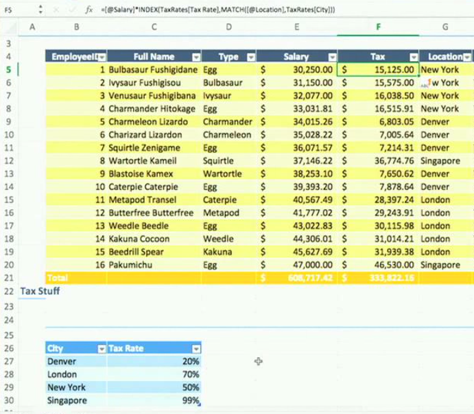
Be sure to sort your lookup table alphabetically by city name (or whatever value you are using MATCH on), otherwise it won’t know how to find what you’re looking for. But that prep is minimal when compared to the time these functions save you.
Interactive Maps Made Easy
Sign Up Now6. BONUS!
While not part of Spolsky’s video, one of our favorite uses of Excel is to store geographic data like addresses and postal codes. Selfishly, the reason we like it for location data is because of the really cool mapping application we’ve been building for the last decade. You can use all the tricks above to organize your data, then simply copy and paste into our mapping tool to generate a map.